

Report :: On the Ideal Fingerboard Scoop Curve

This report is a follow-up (supplementary) study to the previously published "Simulation of Fingerboard Scoop and String Buz" and investigates the shape of the ideal scoop curve. Using the logarithmic spiral, conic sections (parabola, hyperbola, elliptical arc), power curves, and combined curves made by joining these with a sine curve, it examines which curve is the most ideal scoop curve.

1. Overview
This report continues from Sections 4.3 and 4.4 of the previous study (Simulation of Fingerboard Scoop and String Buz") and examines which of several curves is best suited as the scoop curve of the fingerboard.
Starting with the logarithmic spiral, we examined combined curves made by joining a conic section (parabola, hyperbola, elliptical arc) or a power curve with a sine curve. The previous study proposed an asymmetric scoop curve that uses different curves on the nut side and the bridge side; the combined curves in this study are a concrete realization of that idea.
In this study, for the same geometry (fingerboard clearances, position and depth of the scoop vertex, etc.), a curve that satisfies the following conditions is assumed to be the "ideal scoop curve."
Condition 1. Do not carve the fingerboard more than necessary
Condition 2. The maximum amplitude of the string should be larger
Separate condition. The position* and depth of the scoop vertex can be adjusted freely
* Distance along the x-axis measured from the start of the fingerboard
Condition 1 concerns playability and efficiency. To obtain the maximum amplitude, the fingerboard must be carved to some extent, but carving more than necessary only increases the distance between the fingerboard and the string, making the instrument uncomfortable to play. A curve carved only as much as needed keeps the string close to the fingerboard, making it comfortable to play, while also giving a larger maximum amplitude for the stopped string.
Condition 2 is directly related to buzzing: the larger the maximum amplitude, the lower the probability that buzzing occurs. Since the maximum amplitude is divided into the maximum amplitude of the open string and that of the stopped string, the "total maximum amplitude," which is the sum of the two, should be large.
Condition 1 takes priority over Condition 2 because, if the maximum amplitude alone were the criterion, the deeper the fingerboard is dug out, the more advantageous it would be. For example, considering only the open string, carving the fingerboard into an "L" shape would be most advantageous, but this unnecessarily widens the distance between the fingerboard and the string and makes playing difficult. Therefore, we first check whether the fingerboard has been carved efficiently, and then compare the maximum amplitudes.
The separate condition concerns design freedom: if the vertex position and depth cannot be adjusted, the fingerboard shape is restricted accordingly. This condition does not rank the curves; it is a prerequisite for judging whether a curve can be applied to an actual fingerboard.
However, judging whether a curve is ideal also requires evaluation by the player's feel. For practical reasons, such qualitative evaluation was excluded, and only quantitative evaluation items were set as conditions.
This report uses the terminology of the previous study as is. The simulator has been partially modified, but since the modifications do not affect the results of this study, further explanation is omitted.
* For the terms used in the text, please refer to the previous report.
* The principle of the logarithmic spiral is based on the following sources.
- References -
Fisher, A. R. (1969). Curved finger boards for stringed musical instruments (U.S. Patent No. 3,478,631). U.S. Patent and Trademark Office.
Segerman, E. (1993). Fingerboard shapes and graded frets. FoMRHI Quarterly, 71, Comm. 1168, 40–43.
Segerman, E. (1999). Curving a fingerboard to improve the action. FoMRHI Quarterly, 94, Comm. 1621, 37–39.
2. Terms and Concepts
This section explains newly added or important terms and concepts.
■ Maximum Amplitude (Ampmax)
This is the largest amplitude at which the vibrating string does not collide with the fingerboard. It can be divided into the Maximum Open-String Amplitude (O.Ampmax) and the Maximum Stopped-String Amplitude (Ampmax), and the sum of the two is defined as the Total Maximum Amplitude (T.Ampmax).
Since buzzing can occur on both open and stopped strings, a larger "total maximum amplitude," which takes both into account, is better.
In this study, the amplitude of the string is assumed to be proportional to the string length. For a stopped string, moving the stopping point toward the bridge shortens the string and thus reduces the amplitude, so the maximum amplitude cannot be expressed as a single number. Therefore, the maximum amplitude of the stopped string is defined as the amplitude converted to the open-string length.
For example, if the open-string length is 100 and its amplitude is 10, then when the string length at the first stopping point becomes 90, the amplitude at that point becomes 9. According to this proportion, the maximum limit amplitude obtained by converting the stopped-string length to the open-string length is the maximum amplitude of the stopped string.
■ Fingerboard-String Angle (α)
Both ends of an open string are away from the fingerboard, but one end of a stopped string touches the fingerboard because of the finger. The angle formed at the stopping point between the tangent to the fingerboard and the main vibrating portion of the string is defined as the "Fingerboard-String Angle (α)." (Hereafter, angle α) - Fig.2 -

Also, let β be the angle of the envelope endpoint of the main vibrating portion at the stopping point. Since the amplitude is proportional to the string length, angle β is always constant regardless of the position of the stopping point. (Hereafter, angle β) - Fig.3 -

Therefore, if angle β is greater than angle α, a collision occurs. The larger angle α, the larger the maximum amplitude of the stopped string, so if angle α is not constant but varies, the maximum amplitude of the stopped string is determined by its smallest value, the "Minimum Fingerboard-String Angle (αmin)."
■ Angle Variation (|Δα|)
For a stopped string, a curve whose angle α is constant over the entire fingerboard may be the most ideal scoop curve. A constant angle α over the entire fingerboard means that the fingerboard has been carved neither more nor less than needed, and that the curve fully matches the maximum amplitude. From the standpoint of maximum amplitude, this is therefore the most efficient and ideal curve. On an actual violin, however, angle α cannot be constant over the entire fingerboard, so the curve with the smallest variation in angle α (Angle Variation, |Δα|) is the practical ideal curve.
* If two curves have the same |Δα| and αmin, the one with the smaller mean value of angle α is more ideal.
■ Critical Point (Crit.Pos)
For an open string, the point on the fingerboard that the string first touches as its amplitude gradually increases is defined as the "Critical Point (Crit.Pos)." The greater the distance between the fingerboard end and the string, the more the critical point moves toward the nut, and for the same critical point position, the larger the gap between the critical point and the string, the larger the maximum amplitude of the open string.
Since the string and the fingerboard are not parallel, the critical point of the open string lies somewhat toward the nut from the midpoint of the string. The maximum amplitude of the stopped string is determined by αmin, but αmin has no meaning for the open string.
■ Area Factor (AF)
The "Area Factor (AF)" is used as an index for comparing the shapes of curves with the same width and depth. It represents the fullness of a curve (how concave or convex it is) and is defined by the following equation.
Area Factor = Area of the curve / Area of the smallest rectangle enclosing the curve (1)
In other words, AF is the area of the curve when the area of the smallest rectangle enclosing the curve is taken as "1." An AF of 1 means the curve has the same shape as the rectangle, and 0.6 means the curve fills 60% of the rectangle's area. - Fig.4 -
* The Area Factor AF is the same concept as the "Absolute Fullness Index (AFI)" used in the report on violin arching.

The larger the AF, the larger the area of the curve, so the curve can be described as fuller, or as having a higher fullness. AF is therefore used as a parameter to determine the shape when constructing a curve that cannot be defined by width and depth alone, and as a common index when comparing different curves.
■ Combining (Joining) Two Curves
For most curves, the vertex position cannot be changed. To solve this problem, two curves are joined at the vertex. That is, the vertex is used as the joining point, and curves of different widths are used on the left and right sides. If curves of different types are used, a better scoop curve can be created by taking only the advantages of each curve, with the added benefit that the vertex position can be moved freely. The joining point of the two curves becomes the vertex of the scoop, and the two curves must have the same depth.
A curve made by combining a logarithmic spiral, a conic section, or a power curve with a sine curve is defined as a "Combined Curve." However, when the left and right curves are of the same type, it is not called a combined curve but by the name of that curve; the term combined curve is used only when the left and right curves are of different types.
Fig.5 explains how two curves are joined. Two curves of different widths are constructed, each is cut in half, and one half of each is taken and joined together.

However, this method is basically possible only for symmetric curves, so it cannot be applied to the logarithmic spiral. A different method is therefore used for the logarithmic spiral. (See Section 3.2.3)
The point where the two curves are combined (joined) is defined as the "Junction," and the junction is also the vertex of the scoop curve.
For convenience, the section from the junction (scoop vertex) to the nut is referred to as the "Left Curve," and the section from the junction to the bridge-side end as the "Right Curve."
Various curves can be used as the left and right curves, but the simulations are run with the right curve fixed as a sine curve while only the left curve is changed. The reason for choosing the sine curve as the right curve is explained in Section 3.1.
3. Candidate Curves
The curves used in the simulations are as follows.
Sine curve
Logarithmic spiral family: logarithmic spiral, rotated logarithmic spiral, logarithmic-sine combined curve
Conic section family: hyperbola-sine, parabola-sine, ellipse-sine combined curves
Power curve family: power(low)-sine, power(middle)-sine, power(high)-sine combined curves
The sine curve is also used as the right curve of the combined curves.
For conic sections (hyperbola and elliptical arc) and power curves, the fullness of the curve can be adjusted by changing the Area Factor (AF) while keeping the vertex position and depth fixed. For the parabola, once the vertex position and depth are set, there is only one shape, so AF cannot be changed (AF = 2/3). With the parabola as the boundary, the hyperbola and power(low) are less full than the parabola, and the elliptical arc and power(high) are fuller.
* "Low/Middle/High" for power curves only indicates the magnitude of AF, i.e., the degree of fullness.
■ Criteria for Selecting Candidate Curves
Candidates for the left curve of the combined curves were selected based on the following four criteria.
a. The slope at the vertex is zero, and the curve is symmetric about the vertex
: The slope must be zero at the vertex so that the curve joins the sine curve on the right without a kink (C¹ continuity). If the curve is symmetric, it can be cut at the vertex and only one half used, and since the shape of that half is determined only by the half-width and depth, the curves can be compared under the same conditions.
b. The curve changes monotonically from the vertex to the end
: The fingerboard scoop must be a single concave trough. Curves that rise and fall again partway create another undulation within the trough, so they are excluded.
c. Fullness (AF) can be changed continuously while the half-width and depth are fixed
: The fullness of the ideal curve cannot be known in advance. The curve must therefore belong to a family whose fullness can be changed with a single variable, so that the best curve (At) can be found among them.
d. The formula is simple, making calculation and fabrication easy
Based on these criteria, conic sections (hyperbola, parabola, elliptical arc) and power curves were chosen as candidates for the left curve. Both families can change their fullness with a single variable (the cutting range for conics, the exponent for power curves), and both include the parabola (AF = 2/3) in common.
Some curves were included even though they do not satisfy all the criteria.
Logarithmic spiral: It is not symmetric, but it was included as a reference for comparison because it has the ideal property that angle α is constant regardless of the stopping position. In the combined curve, only the part to the left of the vertex is used.
Sine curve: Its fullness is fixed at 2/π, so it does not satisfy criterion c. However, since it is used as the right curve of all combined curves, it was compared as a reference curve.
■ Curves Excluded from the Candidates
Circular arc, cycloid, catenary: Once the half-width and depth are set, the shape is uniquely determined and the fullness cannot be changed (criterion c). Moreover, when the depth is much smaller than the half-width, as in violin-family instruments, they all become almost the same shape as the parabola (AF ≈ 2/3), so they can be represented by the parabola.
Free-form curves such as splines and Bézier curves: They have many shape-defining variables and cannot be organized into a single family of curves, and the results depend on how the variables are chosen, making systematic comparison difficult (criteria c, d).
Below, each curve is briefly described, and from Chapter 4 onward the curves are compared together to find which curve is the most ideal.
3.1. Sine Curve
The sine curve uses a half-period sine waveform as the scoop curve, and its AF is fixed at 2/π ≈ 0.637. Since it is a symmetric curve, the vertex position can be adjusted by joining two sine curves of different half-widths at the vertex.
■ The Sine Curve as the Right Curve
In a normal geometry, angle α in the right curve section gradually increases toward the bridge and reaches its maximum at the fingerboard end. The maximum amplitude is determined by the minimum angle αmin, and αmin is mostly located on the left curve; on the right curve, where the angles are larger than that, the key is to be as close to the string as possible.
Fig.6 shows the hyperbola with minimized AF (Hb), the sine curve (Sn), and the parabola (Pb) used as the right curve. The vertex is at the center of the fingerboard (Gap.3/6 position), and the numbers at Gap.4/6 and 5/6 indicate the gap between the string and the fingerboard. In the figure, the hyperbola (red) is closest to the string. However, it is excessively kinked at the vertex and cannot be used as a fingerboard curve.

Therefore, for the right part of the combined curves, the sine curve was judged to be the most reasonable choice, since it has a narrow gap to the string, joins smoothly at the vertex, and is mathematically simple and easy to construct. The sine curve is used for the right part of all subsequent combined curves.
3.2. Logarithmic Spiral Family
3.2.1. Logarithmic Spiral
A logarithmic spiral is a curve in which, at any point on the spiral, the angle between the straight line connecting that point to the origin and the direction of the spiral is always constant.
If the scoop curve of the fingerboard were a logarithmic spiral, then wherever the fingerboard is stopped, the angle α between the main vibrating portion of the string and the fingerboard tangent at the stopping point would always be constant, and it can be defined by the following equation.
g(r) = α · r · ln( S / r ) (2)
* g(r) : Perpendicular distance from any point on the fingerboard to the open string
* α : Angle between the main vibrating portion of the string and the fingerboard tangent at any point
on the fingerboard (rad)
* r : Distance from the bridge to any point on the fingerboard
* S : String length (from bridge to nut)
Equation (2) above is identical to the equations in the references. However, it assumes that the fingerboard-string gap at the start of the fingerboard (nut) (Clearance at Nut, CLR.Nut) is "0." For the violin this value is not "0," so to apply the logarithmic spiral to a violin fingerboard, the equation must be modified as follows.
g(r) = α · r · ln( A / r ) (3)
A = S · exp( Cn / ( α · S ) ) (4)
* A : Distance from the bridge to the intersection of the spiral and the open string
* Cn : Fingerboard-string gap at the start of the fingerboard (CLR.Nut)
When Cn (= CLR.Nut) is not "0," the intersection of the spiral and the open string is moved from the nut in the direction away from the bridge, so that at the start of the fingerboard (nut) the curve begins with a gap from the string.
However, all the equations above use distances measured from the bridge (bridge x-coordinate = 0). For conceptual consistency, if the nut position is taken as "0" and distances are measured along the x-axis (the straight line connecting the start and end of the fingerboard), the equations become:
g(x) = α · ( P − x ) · ln( ( P + e ) / ( P − x ) ) (5)
e = P · [ exp( Cn / ( α · P ) ) − 1 ] (6)
* g(x) : Perpendicular distance from any point on the fingerboard to the open string
* x : Distance from the nut to any point on the fingerboard (x = 0 at the nut)
* P : Length of the string length S projected onto the x-axis, P = S·F / √( F² + (Cf − Cn)² )
* P − x : Distance from any point on the fingerboard to the bridge
* e : Distance from the nut to the intersection of the spiral and the open string
Angle α can be obtained as follows.
α = ( Cf − u·Cn/P ) / ( u · ln( P/u ) ), u = P − F (7)
* Cf : Fingerboard-string gap at the fingerboard end (CLR.FB)
* F : Fingerboard length
* In violin geometry, the difference between P and S is 0.01% or less, so P ≈ S may be assumed.
■ Characteristics of the Logarithmic Spiral
Fig.7 is an example of applying the above logarithmic spiral to the fingerboard under the reference condition* for the violin's 4th string. It can be seen that wherever the fingerboard is stopped, angle α is always constant at 3.02°. (The graph is vertically exaggerated, so the angle appears larger than the actual 3.02°.)
* Reference condition for the violin's 4th string: string length 330, fingerboard length 270, string gap at fingerboard start/end 0.5/5.5

As shown in Fig.3, for a stopped string the envelope angle β at the stopping point is always constant even when the string length changes as the stopping point moves. Therefore, with a logarithmic spiral the maximum amplitude can be maintained over the entire fingerboard, and the fingerboard-string gap never becomes wider or narrower than necessary in any section. In other words, the logarithmic spiral could be the optimal scoop curve for the fingerboard.
However, the logarithmic spiral also has drawbacks. By its mathematical definition, the vertex position is determined solely by the string and fingerboard lengths, and the vertex depth is determined by the string and fingerboard lengths and by the gaps (clearances) between string and fingerboard at the start and end of the fingerboard. In other words, the vertex position and depth cannot be changed.
Calculating the logarithmic spiral for the 4th-string reference condition,
Vertex position: 152.7mm
Vertex depth: 2.75mm
Angle α: 3.02° (the same over the entire fingerboard)
only one logarithmic spiral is produced.
Unfortunately, these results show that the vertex of the logarithmic spiral is too deep for it to be used as the scoop curve of a violin fingerboard.
Nevertheless, the property of the logarithmic spiral that angle α is constant at every point on the fingerboard can be regarded as a great advantage for a scoop curve. The next section therefore examines the case where the depth of the logarithmic spiral is reduced to the level of an actual instrument so that it can be applied to the fingerboard.
3.2.2. Rotated Logarithmic Spiral
A logarithmic spiral with the desired vertex depth is constructed, and then rotated about the start of the fingerboard so that the gap between the fingerboard end and the string (Clearance at Fingerboard End, CLR.FB) becomes the desired value. The curve completed in this way is defined as the "Rotated Logarithmic Spiral."
For example, if the desired CLR.FB is 5.5 and the vertex depth is 0.7, a logarithmic spiral with a vertex depth of 0.7 is constructed (gray dotted curve) and then rotated so that CLR.FB becomes 5.5 (green solid curve). - Fig.8 -

Since the logarithmic spiral has the property that the larger the gap between the fingerboard end and the string (CLR.FB), the deeper the vertex (they are linked), the curve is first constructed by setting a CLR.FB value that gives the desired vertex depth, and then that curve is rotated to obtain the desired CLR.FB value.
■ Characteristics of the Rotated Logarithmic Spiral
Fig.9 shows angle α of the rotated logarithmic spiral. The angle keeps increasing as the stopping point moves toward the bridge.

In other words, rotating the logarithmic spiral loses the property described as its advantage, namely that "the angle between the string and the fingerboard tangent is constant over the entire fingerboard." Put differently, there is no longer any point in using a logarithmic spiral.
Therefore, if there is a violin that uses a logarithmic spiral as its fingerboard scoop curve, it can only be a rotated logarithmic spiral that has lost the meaning and purpose of the logarithmic spiral, and if the logarithmic spiral was used for the purpose of keeping angle α constant, that was a mistaken judgment.
3.2.3. Logarithmic-Sine Combined Curve
The logarithmic spiral cannot be used because its vertex is too deep, the rotated logarithmic spiral loses its purpose because angle α varies, and neither allows the vertex position to be adjusted.
This section examines the "Logarithmic-Sine Combined Curve," which partly overcomes these problems of the logarithmic spiral.
This curve joins a logarithmic spiral on the nut side (left curve) with a sine curve on the bridge side (right curve), and can be constructed as follows. - Fig.10 -
(A) Draw the open string and a straight fingerboard without scoop
(B) Draw an auxiliary line by offsetting the straight fingerboard downward by the desired vertex depth
(C) Draw a logarithmic spiral that passes through the start of the fingerboard and is tangent to the auxiliary line. (Angle α is constant in all sections, and only one such curve exists.)
(D) Take the point of tangency between the logarithmic spiral and the auxiliary line as the vertex (junction).
(E) Replace the part of the logarithmic spiral to the right of the vertex with a sine curve

In the completed logarithmic-sine combined curve, angle α always has a constant value in the left part and gradually increases in the right part.
Mathematically, it can be constructed as follows.
■ Construction of the Logarithmic-Sine Combined Curve
x is the distance from the nut, and height is measured from the straight line (chord) connecting the start (0, 0) and end (F, 0) of the fingerboard.
a. Logarithmic spiral part (0 ≤ x ≤ Xd)
g(x) = α·(P − x)·ln[ (P + e)/(P − x) ], e = P·[ exp( Cn/(α·P) ) − 1 ] (8)
* g(x): Gap between the string and the fingerboard
* P: Length of the string length S projected onto the x-axis, P = S·F / √( F² + (Cf − Cn)² )
* Cn: String height at the start of the fingerboard
* α: Angle between the fingerboard tangent and the main vibrating portion of the string at the
stopping point (constant)
b. Determining α
P·α·exp[ H/(P·α) − 1 ] = H + D, H = Cn + (Cf − Cn)·P/F (9)
* D : Vertex depth
* H : Height of the open string extended to the bridge
* Cf : String height at the end of the fingerboard
* α is found numerically, and the solution is unique
c. Vertex position
Xd = P − (H + D)/α (10)
* Xd is determined automatically by D (cannot be set separately)
d. Sine curve part (Xd < x ≤ F)
y(x) = −D·sin[ π/2 + (π/2)·(x − Xd)/(F − Xd) ] (11)
* y(x): Fingerboard height (negative on the carved side)
* Quarter period used: −D at Xd, 0 at F
■ Characteristics of the Logarithmic-Sine Combined Curve
In the logarithmic-sine combined curve, the junction is the vertex of the scoop. The logarithmic spiral part has a perfectly constant angle (α), and the sine curve part has the characteristic that the angle gradually increases toward the bridge. As it stands, the logarithmic-sine combined curve might be the ideal scoop curve.
Fig.11 is an actual example of the logarithmic-sine combined curve, and the gray dotted line shows the logarithmic spiral before it was cut.

However, the logarithmic-sine combined curve also has a drawback: the position and depth of the scoop vertex, where the two curves meet, are linked to each other. That is, changing the depth changes the position, and changing the position changes the depth. For example, it is impossible to fix the depth at 1.0 and adjust the position to 115, 135, 155, and so on.

Fig.12 shows the vertex depth and position and the maximum amplitude of the logarithmic-sine combined curve under the violin 4th-string reference condition. For example, if the vertex depth is 0.7, the vertex position must be 105.26, and if the position is to be 135, the depth has to be 1.63. (The blue numbers indicate the amplitude at each point.)
In other words, the vertex position and depth have a one-to-one correspondence, and no combination outside this relationship exists.
Fig.13 and Fig.14 below show angle α in the logarithmic spiral section and the sine curve section, respectively. In the logarithmic spiral section it is constant at 1.86° throughout, and in the sine curve section it gradually increases from 1.86°.
* If the vertex depth exceeds a certain threshold, a section appears in the sine curve part where angle α becomes smaller than the angle in the logarithmic spiral part, so care is needed. The threshold varies with the geometry, but since this occurs only when the vertex is very deep, it need not be a concern in ordinary situations. (This happens because the sine curve is flatter than the cut-off right part of the logarithmic spiral.)
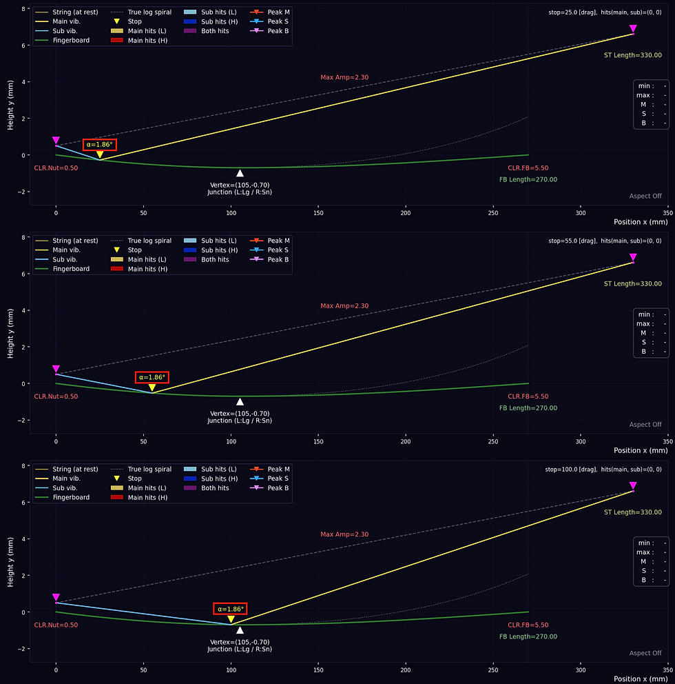

The problems of the logarithmic-sine combined curve can therefore be summarized in two points.
First, the vertex position and depth are linked and cannot be adjusted independently.
Second, angle α is not kept constant in the sine curve section.
However, the second point is a problem that can never be solved geometrically for an instrument with large clearance values such as the violin, so it should be regarded as a characteristic of the instrument rather than a problem.
Therefore, the only remaining problem of the logarithmic-sine combined curve is "the linkage between vertex position and depth," and if there is another curve that does not have this problem and is most similar to the logarithmic spiral, it is very likely to be "the ideal scoop curve of the fingerboard."
The next section examines such candidate curves.
3.3. Conic Section Family
The parabola, hyperbola, ellipse (elliptical arc), and circle (circular arc) are all subcategories of conic sections. They are the cross-sectional curves obtained by cutting a cone with a plane, and the type of curve is determined by the cutting angle.
As in Fig.15, cutting the cone parallel to its base gives a circle, and cutting parallel to the generatrix gives a parabola. Cutting at a shallower angle than the generatrix gives an ellipse, and cutting at a steeper angle than the generatrix gives a hyperbola.
* Generatrix: the straight line running from the apex of the cone to the edge of the base

The sharpness of a cone (the slope of the generatrix) differs from cone to cone, but the type and shape of the curve are determined by how much the cutting plane is inclined relative to the generatrix. Since the same curve can therefore be obtained from any cone, the shape of the cone is not considered further below.
■ How the Curve Is Cut and AF
For the fingerboard scoop, only a portion of these curves near the vertex is cut out and used. First, how far from the vertex to cut is set as a ratio, and the cut piece is then stretched or compressed horizontally and vertically to match the desired half-width and depth. Since AF does not change with stretching or compression, it is determined only by the cutting ratio.
All parabolas are similar to one another, so AF is constant at 2/3 regardless of which section is cut. Therefore, once the half-width and depth are set, the parabola is uniquely determined.
For the hyperbola and the ellipse, AF varies with the cutting ratio. As the section used narrows toward the vertex, both approach the parabola and AF approaches 2/3. With the parabola as the boundary, the ellipse is fuller than the parabola and the hyperbola is less full.
If AF is changed while the half-width and depth are kept the same, the cutting angle also changes accordingly, but it is not the angle that determines AF.
The AF each curve can take is as follows.
Parabola: AF = 2/3 ≈ 0.667 (fixed)
Hyperbola: 0.5 < AF < 2/3
Elliptical arc: 2/3 < AF < π/4
The circle is a special case of the ellipse. Once the half-width and depth are set, it is uniquely determined, and AF takes a value between 2/3 and π/4 depending on the depth/half-width ratio. When the depth is much smaller than the half-width, it is almost identical to the parabola.
In this way, the hyperbola and elliptical arc can change the fullness of the curve by adjusting AF. However, if the entire half-ellipse is used (AF = π/4), the tangents at both ends become vertical, so only a portion of the ellipse near the vertex must be used. For this reason π/4 is excluded from the AF range of the elliptical arc.
In Fig.16, the upper straight line represents the open string, and the two lower curves represent two hyperbolas (fingerboards) with different AF values. One is drawn with the maximum settable AF and the other with the minimum AF, and it can be seen that the larger the AF, the fuller the curve.

Conic sections are also symmetric curves, so the vertex position can be adjusted by joining two curves of different half-widths at the vertex. - Fig.5 -
3.3.1. Conic-Sine Combined Curve
The "Conic-Sine Combined Curve" was devised to solve the "linkage between vertex position and depth" of the logarithmic-sine combined curve.
Depending on the type of left curve, it is divided into the Hyperbola-Sine, Parabola-Sine, and Ellipse-Sine combined curves.
■ Construction of the Conic-Sine Combined Curve
x is the distance from the nut, and height is measured from the straight line (chord) connecting the start (0, 0) and end (F, 0) of the fingerboard.
a. Conic section part (0 ≤ x ≤ Xd)
y(x) = − D/(r − 1) · [ r − √(1 − k·v²) ], v = (x − Xd)/Xd, r = √(1 − k) (12)
* D, Xd: Vertex depth and position (each specified)
* k < 0 hyperbola, k = 0 parabola (y = −D·(1 − v²)), k > 0 elliptical arc
b. Determining k
[ r/2 − Λ(s)/(2s) ] / (r − 1) = A*, s = √|k|, Λ = asinh (k < 0), asin (k > 0) (13)
* A* : Target area factor (default) = hyperbola AFa, parabola AFb, elliptical arc AFc (see Section 4.3)
* (Optimal) Conic-Sine: search within the conic family for the AF that minimizes |Δα|
* k is found numerically, and the solution is unique
c. Calculating the reference area factor AFl (= AFa)
AFa = [ (1 − 3ρ²)/4 − (1 + ln ρ)·(1/2 − ρ) ] / [ (ρ − 1 − ln ρ)·(1 − ρ) ] (14)
ρ = exp[ −1 + (1 − β)·ρ ], β = D/(D + H) (15)
* AFa : Area factor of the logarithmic spiral part (left) of the logarithmic-sine
combined curve under the same conditions
* H : Same as in the logarithmic-sine combined curve
* ρ : Found numerically in 0 < ρ < 1
d. 사인 곡선부 (Xd < x ≤ F)
( Same as the logarithmic-sine combined curve )
3.4. Power Curve Family
The power curve is obtained by replacing the exponent 2 in the parabola y = −D·(1 − v²) with an arbitrary real number p. Since it is not a conic section, there is no concept of cutting a cone or cutting out part of the curve. The same section, from the vertex to the point where y = 0, is always used, and the shape is controlled by the single exponent p.

AF and the exponent p correspond one-to-one through the relation AF = p/(p + 1). When p = 2, the curve is exactly the parabola (AF = 2/3); when p is less than 2, the vertex becomes sharper and the curve less full; and when p is greater than 2, the bottom becomes flatter and the curve fuller. - Fig.17 -
The AF of each range is as follows.
p < 2: 0.5 < AF < 2/3 (Power(Low))
p = 2: AF = 2/3 (Power(Middle), parabola)
p > 2: 2/3 < AF < 1 (Power(High))
The slope at both ends, p·D/half-width, is always finite, so there is no constraint like the ellipse's vertical end tangents. Therefore, AF values greater than π/4, which the conic family cannot exceed, can also be produced (program upper limit 0.900, p = 9). Conversely, if p ≤ 1 (AF ≤ 0.5), the slope at the vertex does not become zero and the curve is kinked, so it cannot be used.
Even with the same AF, power curves and conic sections have different shapes, so the two families are treated as different curves.
As with conic sections, the vertex position can be adjusted by joining two curves of different half-widths at the vertex.
3.4.1. ower-Sine Combined Curve
The Power-Sine Combined Curve replaces the left curve of the conic-sine combined curve with a power curve, and according to AF it is divided into the Power(Low)-Sine, Power(Middle)-Sine, and Power(High)-Sine combined curves.
■ Construction of the Power-Sine Combined Curve
x is the distance from the nut, and height is measured from the straight line (chord) connecting the start (0, 0) and end (F, 0) of the fingerboard.
a. Power curve part (0 ≤ x ≤ Xd)
y(x) = − D·(1 − |v|^p), v = (x − Xd)/Xd (16)
* D, Xd: Vertex depth and position (each specified)
* p = 2: parabola
b. Determining p
p = A*/(1 − A*) (17)
* A* : Target area factor (default) = Power(Low) AFa, Power(Middle) AFb,
Power(High) AFc (see Section 4.3)
* (Optimal) Power-Sine: search within the power family for the AF that minimizes
|Δα| (0.5 < AF ≤ 0.900)
* No numerical solution needed (closed form)
c. Calculating the reference area factor AFl (= AFa)
( Same as the conic-sine combined curve )
d. Sine curve part (Xd < x ≤ F)
( Same as the logarithmic-sine combined curve )
4. Comparison Method
4.1. Comparison Conditions
All curves are compared under the following common geometry.
String length 330, fingerboard length 270
String gap at fingerboard start/end: 1st string 0.3/3.5, 4th string 0.5/5.5
Vertex depth: 1st string 0.3, 4th string 0.7
* For accurate comparison, the "Exclusion Zone (Excl Zone)" was set to "0." Since this setting differs from the previous study (±10mm), the maximum amplitude values come out slightly smaller even under the same conditions.
The curves are compared at predetermined comparison points (Section 4.2), and whether the results also hold under other conditions is checked with the simulator's Amplitude & |Δα| Map. There are two kinds of maps. The vertex depth–position map varies the vertex depth and position with CLR.FB fixed, and the vertex depth–CLR.FB map varies the vertex depth and CLR.FB with the vertex position fixed (at 135mm, the center of the fingerboard, in this study).
4.2. Comparison Steps
In the logarithmic-sine combined curve, the vertex depth and position are linked, so it exists only at specific combinations; these are defined as the "Special Combination." The comparison is therefore carried out in the following two steps, with the 1st and 4th strings compared separately in each step.
Step | String 1 (Vertex Depth 0.3) | String 4 (Vertex Depth 0.7) |
Step 1: Special Combination | Vertex Position 91.94 | Vertex Position 105.26 |
Step 2: General Positions | Vertex Position 115 / 135 / 155 | |
Table 1: Comparison Steps and Vertex Positions
Step 1 is the only position where the logarithmic-sine combined curve exists. Since the logarithmic-sine combined curve has a constant angle α over the entire left section, a curve that performs closer to the logarithmic-sine combined curve under this condition is more likely to be the ideal curve.
Step 2 is the condition in which the vertex is moved at the same depth. Since the logarithmic-sine combined curve cannot exist at these positions, it is excluded from the comparison, and the best curve among the remaining curves is sought.
4.3. Classification of Curves
For the curves whose fullness can be adjusted, AF was set based on the AF of the logarithmic spiral part of the logarithmic-sine combined curve (AFl), and the curves were classified as follows.
* Abbreviation : Sn=Sine, Lg=Logarithmic, Cn=Conic, Hb=Hyperbola, Pb=Parabola, Ep=Ellipse, Pw=Power, Lo=Low, Md=Middle, Hi=High, At=Auto, C□=Conic Hb/Pb/Ep, P□=Power Lo/Md/Hi
Group | Curve | Notation | AF of the Left Curve |
|---|---|---|---|
Base | Sine (Sine-Sine) | Sn | AFs = 2/π ≈ 0.637 (fixed) |
Logarithmic-Sine | Lg | AFl = AF of the log-spiral section (variable) | |
Group a | Hyperbola-Sine Power(Low)-Sine | Cn-Hb Pw-Lo | AFa = AFl (variable) |
Group b | Parabola-Sine Power(Middle)-Sine | Cn-Pb Pw-Md | AFb = 2/3 ≈ 0.667 (fixed) |
Group c | Ellipse-Sine Power(High)-Sine | Cn-Ep Pw-Hi | AFc = AFb+(AFb-AFa) (variable) |
Group d | (Optimal) Conic-Sine (Optimal) Power-Sine | At-C□ At-P□ | AFd = AF with the minimum |Δα| (variable) |
Table 2: Classification of Curves
The base group consists of the curves that serve as the reference for the overall comparison.
Group a uses the AF of the logarithmic spiral part as is, and group c has AF values symmetric to those of group a about group b (2/3). The Power(Middle)-Sine combined curve is a parabola with exponent p = 2, so it is the same curve as the Parabola-Sine combined curve.
AFl (= AFa) varies with the geometry and vertex depth, so the AF of groups a and c changes along with it. AFd additionally varies with the vertex position.
There is no guarantee that the AF of the ideal curve exactly matches the values of groups a, b, and c. Therefore, for the conic-sine and power-sine combined curves, the AF that minimizes |Δα| within each family was searched automatically, and these were placed in group d.
■ Notation of Group d (At-□□)
The curve names of groups a, b, and c (Cn-Hb, Pw-Lo, etc.) are also the names of AF ranges. For example, the Hyperbola-Sine (Cn-Hb) is one curve, with AF = AFa, selected from the many curves belonging to the hyperbola range where AF is less than 2/3.
Group d (At) is a single curve obtained by finding the AF with the smallest |Δα| over the entire search range of each family. Two letters are appended according to which range the found AF falls in.
Family | Search Range | AF < 2/3 | AF = 2/3 | AF > 2/3 |
Conic (At-C□) | 0.505 ~ 0.780 | At-CH (Hyperbola side) | At-CP (Parabola) | At-CE (Ellipse side) |
Power (At-P□) | 0.505 ~ 0.900 | At-PL (Low side) | At-PM (Middle) | At-PH (High side) |
Table 3: Notation of the Optimal Curves (At-□□)
Thus At-CH and Cn-Hb are curves in the same hyperbola range, but with different AF values.
At-CH has the AF that minimizes |Δα|, while Cn-Hb has AFa. The last two letters only indicate "which range the search result came from," and do not denote a separate type of curve.
4.4. Evaluation Items
The three conditions of Chapter 1 are evaluated with the following items.
Condition | Indicator |
|---|---|
Condition 1 (Carving Efficiency) | Angle Range (|Δα|) |
Condition 2 (Maximum Amplitude) | Total Maximum Amplitude (T.Ampmax) |
Separate Condition (Design Freedom) | Vertex position and depth can be set independently |
Table 4: Evaluation Criteria
Condition 1: Since the maximum amplitude of the stopped string is determined at the single point of αmin, sections where angle α is greater than αmin are carved more than necessary. |Δα| represents the size of this excess, and 0 means that every stopping point is carved only as much as needed. In other words, Condition 1 evaluates not the distance to the string itself, but the efficiency of carving the fingerboard relative to the maximum amplitude.
* When the vertex position and depth are the same, the mean of angle α over the left section is nearly the same, so a smaller |Δα| means a larger αmin, which is also advantageous for the total maximum amplitude.
Condition 2: Since buzzing occurs on both open and stopped strings, the total maximum amplitude, the sum of the two maximum amplitudes, is used as the indicator. The maximum amplitude of the open string is determined by the fingerboard-string gap at the critical point, and that of the stopped string by the minimum angle αmin. The total maximum amplitude therefore reflects both factors.
The separate condition is satisfied by all curves except the logarithmic-sine combined curve. Since the logarithmic-sine combined curve does not satisfy this condition, it is used only as a reference curve for comparison.
Therefore, the curve with the smallest |Δα| is given priority, and when the |Δα| values are similar, within 0.001°, the curve with the larger total maximum amplitude is judged to be superior.
5. Comparison Results
This chapter compares the angle variation (|Δα|) and total maximum amplitude (T.Ampmax) of each curve according to the conditions and steps of Chapter 4.
5.1. Comparison Points and Notation
Fig.18 marks the points used for this comparison on the vertex depth–position plane (left: 1st string, right: 4th string). The light blue line represents the combinations of vertex depth and position at which the logarithmic-sine combined curve can exist (Special Combination).
The Step 1 comparison points (red circles) lie on this line, with vertex depths of 0.3 for the 1st string and 0.7 for the 4th string, and vertex positions of 91.94 and 105.26, respectively. The Step 2 comparison points (blue squares) move the vertex position to 115, 135, and 155mm at the same depth; all of them lie off this line, so they are conditions under which the logarithmic-sine combined curve cannot exist.

In the comparison tables below, the reference curve is shown in green, and the best value in each column is shown in red. Smaller |Δα| and larger T.Ampmax are better.
The ranking of curves follows the judgment rule of Section 4.4, and AF values are shown alongside so that it can be seen which curve the optimal curve is.
5.2. Step 1: Special Combination
In Step 1, all curves were compared at the vertex positions where the logarithmic-sine combined curve exists (1st string 91.94, 4th string 105.26). This is the only condition under which the logarithmic-sine combined curve, which is closest to the ideal curve, can be compared directly with the other curves, and it is intended to confirm what the optimal curves (group d) mean.
Group | Curve | String 1 | String 4 | ||||
|Δα| | T.Ampmax | AF | |Δα| | T.Ampmax | AF | ||
Base | Logarithmic-Sine (Lg) | 0.000 | 3.65 | 0.658 | 0.000 | 6.26 | 0.656 |
Sine (Sn) | 0.075 | 3.58 | 0.637 | 0.145 | 6.13 | 0.637 | |
Group a | Hyperbola-Sine (Cn-Hb) | 0.006 | 3.64 | 0.658 | 0.015 | 6.25 | 0.656 |
Power(Low)-Sine (Pw-Lo) | 0.006 | 3.65 | 0.658 | 0.015 | 6.25 | 0.656 | |
Group b | Parabola-Sine (Cn-Pb) Power(Middle)-Sine (Pw-Md) | 0.026 | 3.64 | 0.667 | 0.061 | 6.25 | 0.667 |
Group c | Ellipse-Sine (Cn-Ep) | 0.059 | 3.63 | 0.676 | 0.141 | 6.23 | 0.677 |
Power(High)-Sine (Pw-Hi) | 0.047 | 3.63 | 0.676 | 0.113 | 6.23 | 0.677 | |
Group d | Optimal Conic-Sine (At-Cn) | 0.003 | 3.65 | 0.659-H | 0.008 | 6.25 | 0.657-H |
Optimal Power-Sine (At-Pw) | 0.005 | 3.65 | 0.656-L | 0.011 | 6.25 | 0.655-L | |
Table 5: Comparison at the Special Combination (Step 1)
■ Angle Variation |Δα|
For both strings, |Δα| increases in the order group d < group a < group b < group c < sine curve. That is, the farther the AF of the left curve is from the AF of the logarithmic spiral part (AFl), the larger |Δα|.
The curve with the smallest |Δα| for both strings is the Optimal Conic-Sine combined curve (At-CH) (1st string 0.003°, 4th string 0.008°). The Optimal Power-Sine combined curve (At-PL) is next smallest, but the difference exceeds the judgment criterion (0.001°), so At-CH is the best.
Within the same group, in group c the Power(High)-Sine has a smaller |Δα| than the Ellipse-Sine even with the same AF. In group a there is no difference between the two curves. This shows that even with the same AF, |Δα| can differ depending on the shape of the curve.
■ Total Maximum Amplitude T.Ampmax
For groups a, b, and d, T.Ampmax is almost the same as that of the logarithmic-sine combined curve, within 0.01. In contrast, group c is 0.02–0.03 smaller and the sine curve 0.07–0.13 smaller. Curves with larger |Δα| tend to have smaller T.Ampmax, confirming that, as explained in Section 4.4, a curve with a small |Δα| is also advantageous in total maximum amplitude.
■ AF of the Optimal Curves
The AF of the optimal curves is almost the same as the AF of the logarithmic spiral part (AFl).
1st string : AFl 0.658 / At-CH 0.659 / At-PL 0.656
4th string : AFl 0.656 / At-CH 0.657 / At-PL 0.655
In other words, at the special combination the curve with the smallest |Δα| has almost the same fullness as the logarithmic spiral part. Since the logarithmic spiral is a curve with constant angle α, the closer the fullness, the closer the angle distribution is to that of the logarithmic spiral. Interestingly, the optimum of the conic family is slightly larger than AFl, and that of the power family slightly smaller. Depending on the shape of the curve, the optimum falls on either side of AFl.
■ Distribution of Angle α
Fig.19 shows the distribution of angle α for the base group and group d curves on the 4th string. The logarithmic-sine combined curve appears as a horizontal line, with angle α perfectly constant from the start of the fingerboard to the vertex (junction). The sine curve starts at a low value, increases, and then decreases again, showing a large variation. The two group d curves show only very slight variation near the logarithmic-sine combined curve.
* The power(low) curve has a sharply increasing curvature near the vertex, so angle α changes abruptly just before the vertex.

■ Step 1 Conclusion
At the special combination, the optimal curves (group d) give the results closest to the logarithmic-sine combined curve, and At-CH is the best for both strings. Neither conic sections nor power curves can perfectly reproduce the logarithmic spiral, so |Δα| does not become 0, but the difference is very small.
Groups a, b, and c, being single points on the AF axis, cannot be better than the optimal curve of their family. Therefore, in the Step 2 comparison that follows, only the base group (sine curve) and group d are compared.
5.3. Step 2: Vertex Positions 115 / 135 / 155mm
In Step 2, the vertex position was moved to 115, 135, and 155mm at the same vertex depth as in Step 1 (1st string 0.3, 4th string 0.7). All these positions are off the special combination toward the bridge, so the logarithmic-sine combined curve cannot exist there. The curves compared are the sine curve of the base group and the two optimal curves of group d, with the sine curve as the reference curve.
Curve | Vertex Position 115 | Vertex Position 135 | Vertex Position 155 | ||||||
|Δα| (°) | T.Ampmax | AF | |Δα| (°) | T.Ampmax | AF | |Δα| (°) | T.Ampmax | AF | |
Sine (Sn) | 0.234 | 3.46 | 0.637 | 0.391 | 3.37 | 0.637 | 0.567 | 3.30 | 0.637 |
Optimal Conic-Sine (At-Cn) | 0.147 | 3.58 | 0.687-E | 0.290 | 3.53 | 0.705-E | 0.457 | 3.49 | 0.718-E |
Optimal Power-Sine (At-Pw) | 0.133 | 3.61 | 0.709-H | 0.263 | 3.59 | 0.745-H | 0.419 | 3.58 | 0.773-H |
Table 6: Comparison at Vertex Positions 115 / 135 / 155 mm (Step 2, String 1)
Curve | Vertex Position 115 | Vertex Position135 | Vertex Position 155 | ||||||
|Δα| (°) | T.Ampmax | AF | |Δα| (°) | T.Ampmax | AF | |Δα| (°) | T.Ampmax | AF | |
Sine (Sn) | 0.250 | 6.00 | 0.637 | 0.528 | 5.79 | 0.637 | 0.831 | 5.63 | 0.637 |
Optimal Conic-Sine (At-Cn) | 0.107 | 6.20 | 0.669-E | 0.352 | 6.09 | 0.689-E | 0.632 | 5.98 | 0.704-E |
Optimal Power-Sine (At-Pw) | 0.102 | 6.22 | 0.676-H | 0.321 | 6.16 | 0.713-H | 0.578 | 6.13 | 0.744-H |
Table 7: Comparison at Vertex Positions 115 / 135 / 155 mm (Step 2, String 4)
■ Angle Variation |Δα|
At all positions on both strings, |Δα| is in the order Optimal Power-Sine < Optimal Conic-Sine < sine curve. The difference between At-PH and At-CE is 0.005–0.054°, all exceeding the judgment criterion (0.001°), so the Optimal Power-Sine combined curve is the best under all Step 2 conditions.
As the vertex moves farther toward the bridge, |Δα| of all curves increases, and the difference between the two optimal curves also grows. Compared with Step 1 (special combination), where |Δα| was 0.01° or less, it can be seen that once off the special combination, it is difficult for any curve to keep angle α constant.
■ Total Maximum Amplitude T.Ampmax
T.Ampmax follows the same order as |Δα|, and the Optimal Power-Sine combined curve is the largest under all conditions. It is 0.15–0.28 larger than the sine curve on the 1st string and 0.22–0.50 larger on the 4th string, and the difference grows as the vertex moves toward the bridge.
There is a reason why the rankings of |Δα| and T.Ampmax match perfectly in Step 2. Since the slope of the fingerboard is zero at the vertex, angle α at the vertex is the same regardless of the type of curve (the point where all curves meet on the vertical line at the vertex in Fig.20). When the vertex is on the bridge side of the special combination, the place where α is largest in the left section is the vertex, so |Δα| becomes "α at the vertex − αmin." Therefore, a small |Δα| means a large αmin, and a large αmin means a large maximum amplitude for the stopped string.
■ AF of the Optimal Curves
In Step 1, the AF of the optimal curves was almost the same as the AF of the logarithmic spiral part (about 0.656–0.658, in the hyperbola/power(low) range). In Step 2, by contrast, it moves to the elliptical arc/power(high) range above 2/3 under all conditions, and the AF becomes larger as the vertex moves toward the bridge. This is because, as the vertex moves toward the bridge, a fuller curve is needed to maintain the gap to the string over the long left section on the nut side.
Here the AF of the power curve is always larger than that of the conic section (up to 0.773), and the difference also grows as the vertex moves away. Conic sections can produce AF only up to around π/4, and even at the same AF the power(high) curve has a smaller |Δα| than the elliptical arc (group c in Section 5.2). These two factors combine to give the Optimal Power-Sine combined curve the better results.
■ Distribution of Angle α
Fig.20 and 21 show the distribution of angle α for the three curves at the vertex position of 135mm (left section enlarged). The sine curve has the smallest α at the start of the fingerboard and keeps increasing up to the vertex, giving the largest variation. The two optimal curves raise α on the fingerboard-start side to reduce the overall variation, and the Optimal Power-Sine combined curve has the highest αmin and the flattest distribution over most of the left section.


■ Step 2 Conclusion
Under all conditions off the special combination (two strings × three positions), the Optimal Power-Sine combined curve (At-PH) is the best in both |Δα| and T.Ampmax. Its advantage grows as the vertex moves farther from the special combination.
5.4. Summary: Conic vs Power
The results of the two optimal curves (At-Cn, At-Pw) under the eight comparison conditions of Sections 5.2 and 5.3 are summarized in Table 8.
String | Vertex Position | At-Cn |Δα| (AF) | At-Pw |Δα| (AF) | Better | |
Step 1 | 1 | 91.94 | 0.003 (0.659-H) | 0.005 (0.656-L) | Conic |
4 | 105.26 | 0.008 (0.657-H) | 0.011 (0.655-L) | Conic | |
Step 2 | 1 | 115 | 0.147 (0.687-E) | 0.133 (0.709-H) | Power |
135 | 0.290 (0.705-E) | 0.263 (0.745-H) | Power | ||
155 | 0.457 (0.718-E) | 0.419 (0.773-H) | Power | ||
4 | 115 | 0.107 (0.669-E) | 0.102 (0.676-H) | Power | |
135 | 0.352 (0.689-E) | 0.321 (0.713-H) | Power | ||
155 | 0.632 (0.704-E) | 0.578 (0.744-H) | Power |
Table 8: Summary of Comparison between the Optimal Conic-Sine and Power-Sine Combined Curves (All results were decided by |Δα|)
Under all conditions, the difference in |Δα| exceeded the judgment criterion (0.001°), so the judgment was made by |Δα|. T.Ampmax is also equal or larger under all conditions for the curve judged superior by |Δα|.
■ Results at the Comparison Points
At the special combination (Step 1), the Optimal Conic-Sine combined curve (At-CH) is superior, but the difference is very small, 0.001–0.003° in |Δα|, and T.Ampmax is the same. In contrast, at all positions off the special combination (Step 2), the Optimal Power-Sine combined curve (At-PH) is superior. It is better by 0.005–0.054° in |Δα| and by 0.02–0.15 in T.Ampmax, and the difference grows as the vertex moves farther from the special combination.
■ Results over the Entire Range
To check whether the same conclusion holds between and beyond the comparison points, the two optimal curves were compared at all combinations of vertex depth and position. Fig.22 and Fig.23 are drawn in Best Curve mode of the simulator's Amplitude & |Δα| Map (hereafter the Best Curve map). Green indicates the region where the Optimal Conic-Sine combined curve is superior, blue the region where the Optimal Power-Sine combined curve is superior, and the darker the color, the larger the difference in |Δα| between the two curves.


The region where the Optimal Conic-Sine combined curve is superior is only a narrow green band just to the right of the line where the logarithmic-sine combined curve exists (the special combination), and even within this band the difference between the two curves is small (light color). In all other regions, both to the left (nut side) and to the right (bridge side) of the line, the Optimal Power-Sine combined curve is superior, and the difference widens considerably with distance from the special combination (dark color). A typical violin fingerboard places the vertex near the center of the fingerboard, so most fingerboards fall in this region.
■ Results on the Vertex Depth–CLR.FB Plane
With the vertex position fixed at 135mm, the two optimal curves were compared while varying the vertex depth and CLR.FB (Fig.24, 25). Since changing CLR.FB also changes the vertex position of the logarithmic-sine combined curve, a special combination giving a vertex position of 135mm also exists on this plane, running diagonally.


The results are the same as on the vertex depth–position plane. The region where the Optimal Conic-Sine combined curve is superior is only a narrow band lying diagonally along this special combination (e.g., CLR.FB of about 2.5–3.0mm at a depth of 0.7), and in all other regions the Optimal Power-Sine combined curve is superior. The results for the two strings are also almost the same. The typical CLR.FB of a violin (about 3.5mm for the 1st string, about 5.5mm for the 4th string) and vertex depth lie outside this band, so the Optimal Power-Sine combined curve is superior on this plane as well.
■ Why the Power Curve Is Superior
Off the special combination, the AF of the optimal curve moves to the range above 2/3 (elliptical arc/power(high)). In this range, the power(high) curve has a smaller |Δα| than the elliptical arc even at the same AF (group c result in Section 5.2). In addition, conic sections can produce AF only below π/4, whereas power curves have no such constraint. For these two reasons, the advantage of the power curve grows as the vertex moves farther from the special combination.
This is in the same direction as the result of the previous study that a curve closer to a U shape is more advantageous when the vertex is near the center of the fingerboard. However, fuller is not always better; there is an optimal fullness at which |Δα| is minimized, depending on the vertex position and depth.
■ Overall Conclusion
Both optimal curves are superior to the other curves, and at the special combination, where the logarithmic-sine combined curve exists, they give almost the same results as the logarithmic-sine combined curve.
In the narrow band of the special combination, the Optimal Conic-Sine combined curve is slightly superior, but the difference is small enough to be negligible.
In almost all other regions, that is, at most positions where the vertex can be placed on an actual instrument, the Optimal Power-Sine combined curve is the best in both |Δα| and total maximum amplitude.
This result holds not only on the vertex depth–position plane but also when the vertex position is fixed and CLR.FB is varied.
Therefore, by the evaluation criteria of this study (|Δα|, total maximum amplitude, and whether the vertex position and depth can be adjusted), under most conditions other than the special combination, the curve closest to "the ideal scoop curve of the fingerboard" is the Optimal Power-Sine combined curve, with AF (exponent p) chosen so that |Δα| is minimized under those conditions.
6. Discussion
6.1. Verification on the Viola and Cello
5장에서To check whether the conclusions of Chapter 5 also hold for other instruments, the same method was applied to the viola and cello. The calculation conditions are as follows.
Viola: string length 380, fingerboard length 305
1st string: CLR.Nut / CLR.FB 0.4 / 3.5, vertex depth 0.5
4th string: CLR.Nut / CLR.FB 0.8 / 5.5, vertex depth 0.9
Vertex positions: special combination, fingerboard center (152.5), center ±25mm
Cello: string length 695, fingerboard length 580
1st string: CLR.Nut / CLR.FB 0.6 / 5.0, vertex depth 0.7
4th string: CLR.Nut / CLR.FB 1.0 / 7.0, vertex depth 1.6
Vertex positions: special combination, fingerboard center (290), center ±40mm
The results are the same as for the violin.
Special combination: In all four cases the Optimal Conic-Sine combined curve is slightly superior, but the difference in |Δα| between the two optimal curves is very small, 0.001–0.003°. The total maximum amplitude is almost the same as that of the logarithmic-sine combined curve (difference 0.01 or less).
Other positions: Except for one location very close to the special combination, the Optimal Power-Sine combined curve is superior at all positions. This holds on both the nut side and the bridge side of the special combination, and the difference grows with distance from the special combination. For example, at center +25mm on the viola 4th string, the differences are 0.04° in |Δα| and 0.12 in total maximum amplitude.
Exceptions: At 127.5mm on the viola 1st string, only 2mm from the special combination (125.3mm), the conic curve was superior.
At center −40mm (250mm) on the cello 4th string, |Δα| was clearly smaller for the Optimal Power-Sine combined curve (0.051° vs 0.075°), but the total maximum amplitude was 0.03 larger for the Optimal Conic-Sine combined curve. In this case, the power curve was judged superior according to the priority of Section 4.4 (|Δα| first).
Position of the special combination: When the vertex is deep, as on the cello 4th string, the special combination (267mm) comes close to the fingerboard center (290mm). As a result, the difference between the two optimal curves was small even at the center (|Δα| 0.0014°). Even so, the power curve is superior.
Therefore, on the viola and cello as well, the Optimal Power-Sine combined curve is the best at most vertex positions except near the special combination.
6.2. Vertex Depth and Position Giving the Same Maximum Amplitude
When a curve is selected in the Amplitude & |Δα| Map, the maximum amplitude of that curve is displayed as contour lines. All combinations on the same contour have the same maximum amplitude, so this map allows the fingerboard dimensions to be chosen more freely while maintaining the maximum amplitude. The slope of the contours also shows which value has a greater effect on the maximum amplitude. The following results were obtained from the map with the Optimal Power-Sine combined curve (At-Pw) selected.
On the vertex depth–position map, making the vertex 0.1mm deeper increases the total maximum amplitude by about 0.2 (1st string 0.22, 4th string 0.20–0.22). In contrast, the change with vertex position is much smaller, so the maximum amplitude is determined mainly by the vertex depth.
The previous study confirmed that with a parabolic scoop, the maximum amplitude is greatest when the vertex is at about 1/3 of the fingerboard, and decreases greatly as the vertex moves toward the bridge. The trend is the same for the Optimal Power-Sine combined curve: the total maximum amplitude is greatest near the special combination (105.26mm at depth 0.7 on the 4th string) and decreases toward the bridge.
However, since the optimal curve has its AF adjusted for each vertex position, the decrease is small. When the vertex is moved from 105.26mm to 155mm, the parabola loses 0.43, whereas the Optimal Power-Sine combined curve loses only 0.12. On the other hand, |Δα| depends strongly on the vertex position, increasing by about 0.06–0.13° for every 10mm the vertex moves toward the bridge.
Therefore, from the standpoint of both maximum amplitude and |Δα|, it is advantageous to place the vertex on the nut side, close to the special combination, rather than toward the bridge, which agrees with the conclusion of the previous study. The maximum amplitude is then adjusted mainly by the vertex depth.
6.3. Vertex Depth and CLR.FB Giving the Same Maximum Amplitude
The previous study confirmed that with a parabolic scoop there are multiple combinations of fingerboard clearance and vertex depth that give the same maximum amplitude. Here the same relationship is checked on the vertex depth–CLR.FB map (vertex position 135mm) with the Optimal Power-Sine combined curve (At-Pw) selected.
Raising CLR.FB by 0.5mm increases the total maximum amplitude by about 0.38–0.40, and making the vertex 0.1mm deeper increases it by about 0.2. That is, 0.1mm of vertex depth has the same effect as about 0.26–0.28mm of CLR.FB, and the contours of this map show the trade-off relationship between the two values.
String | Vertex Depth / CLR.FB | T.Ampmax | |Δα| |
1 | 0.3 / 3.5 | 3.59 | 0.263 |
0.5 / 3.0 | 3.62 | 0.132 | |
4 | 0.7 / 5.5 | 6.16 | 0.321 |
0.9 / 5.0 | 6.17 | 0.197 |
Table 9: Combinations of Vertex Depth and CLR.FB with Nearly Equal Maximum Amplitude (Vertex Position 135)
For example, on the 4th string, using 0.9/5.0 instead of 0.7/5.5 keeps the total maximum amplitude the same while lowering the string height at the fingerboard end by 0.5mm, and |Δα| also becomes smaller. On the 1st string, using 0.5/3.0 instead of 0.3/3.5 gives the same result.
However, increasing the vertex depth means that the fingerboard is curved that much more, and changing CLR.FB changes the geometry of the whole instrument. This map should therefore be used not as a source of the right answer, but as a reference for balancing playability (string height) against the amount of carving (depth) within the same maximum amplitude.
6.4. Limitations of the Study
The results of this study were obtained within the following assumptions and scope.
Amplitude model: The amplitude of the string was assumed to be proportional to the string length. In actual string vibration, the stiffness of the string, damping, and the position and pressure of the bow also play a role. The results are therefore meaningful for comparing which curve gives a larger amplitude, rather than for the maximum amplitude values themselves.
Fingerboard shape: Only the longitudinal section of the fingerboard (the scoop curve) was considered. The transverse curvature of the fingerboard (radius) and the height differences between strings were not considered.
Right curve: The right curve of all combined curves was fixed as a sine curve (Section 3.1). This has almost no effect on the maximum amplitude, but it does affect the string height between the vertex and the fingerboard end (the right curve).
Judgment criterion: The optimal curve (At) was found using only the |Δα| of the stopped string; the open string was reflected only through the total maximum amplitude.
Exclusion zone: To see the differences between curves precisely, the exclusion zone was set to 0. In actual playing, minute collisions right next to the stopping point are not audible, so the absolute value of the maximum amplitude is calculated slightly smaller than in reality.
Qualitative evaluation: Evaluation by the player's feel was not included.
Machining precision: Some of the differences between curves (|Δα| of 0.01° or less, maximum amplitude of 0.01–0.02) are smaller than the machining precision of an actual fingerboard. Such differences are properly regarded as theoretical rankings only.
7. Conclusion
In this study, the conditions for the ideal scoop curve were defined as not carving the fingerboard more than necessary (|Δα|), a large maximum amplitude of the string (total maximum amplitude), and the ability to set the vertex position and depth freely, and several candidate curves were compared.
The logarithmic spiral has the ideal property that angle α is constant at every stopping point, but its vertex is too deep for it to be used as is. Rotating it loses this property. The logarithmic-sine combined curve preserves this property in the left section of the fingerboard, but since its vertex position and depth are bound to each other, it exists only at specific combinations (the special combination).
For the conic-sine and power-sine combined curves, which allow the vertex position and depth to be set freely, the optimal curve minimizing |Δα| was found within each family and compared, with the following results.
At the special combination, both optimal curves give almost the same results as the logarithmic-sine combined curve, and the fullness (AF) of the optimal curves is almost the same as that of the logarithmic spiral part. Of the two, the Optimal Conic-Sine combined curve is slightly superior, but the difference is small enough to be negligible.
Under most conditions off the special combination, the Optimal Power-Sine combined curve is the best in both |Δα| and total maximum amplitude, and the difference grows with distance from the special combination. This result is the same on both the vertex depth–position plane and the vertex depth–CLR.FB plane, and also on the viola and cello.
When the vertex is near the center of the fingerboard, the optimal curve moves to the side fuller than the parabola (AF > 2/3). This is in the same direction as the result of the previous study that a curve closer to a U shape is advantageous. However, fuller is not always better; an optimal fullness exists for each condition.
Therefore, by the evaluation criteria of this study, under most conditions other than the special combination, the curve closest to the ideal scoop curve is the Optimal Power-Sine combined curve, with the exponent p chosen so that |Δα| is minimized under those conditions.
Regarding fingerboard dimensions, the following was confirmed.
The total maximum amplitude is determined mainly by the vertex depth, and the effect of the vertex position is relatively small. In contrast, |Δα| depends strongly on the vertex position. From the standpoint of both maximum amplitude and |Δα|, it is advantageous to place the vertex on the nut side, close to the special combination, rather than toward the bridge, which agrees with the conclusion of the previous study.
0.1mm of vertex depth has the same maximum-amplitude effect as about 0.26–0.28mm of fingerboard clearance (CLR.FB). Therefore, making the vertex slightly deeper allows the string height at the fingerboard end to be lowered while maintaining the same maximum amplitude.
Using the simulator's Amplitude & |Δα| Map, one can see at a glance which curve is advantageous for a given geometry (Best Curve map) and which combinations of dimensions give the same maximum amplitude (contour lines).
The results of this study are based on a simplified amplitude model and quantitative indicators. Their effect on an actual fingerboard needs to be confirmed through evaluation by players.
Comments